Phyloseq analysis template

library(RauENVS)
library(tidyverse)
library(phyloseq)
library(microbiome)
library(cowplot)
library(vegan)
library(magrittr)
set_theme_AU_ENVS()
data("phyloseq_template_toy_data")

This is a RMarkdown template for doing a quick analysis of an OTU and taxonomic table using RMarkdown.

It contains toy data to illustrate what this notebook does. First, make sure you run the entire notebook with the toy example. To do this, click on “Knit” in Rstudio.

Read your data

You need 3 tabulated files with contains metadata, OTU and taxonomy, respectively. Please make sure you read the data correctly. Delete the code that generates the toy example and uncomment the code that reads files.

Read metadata table

You metadata table must contain a column named rowname and as many features as desired. Either edit the tabulated file or rename the column with the sample identifier. Your metadata table should look something like the example below.

By assigning a variable inside () we print a summary.

# (metadata_tbl <- readr::read_csv("metadata_dummy.csv"))
metadata_tbl <- phyloseq_template_toy_data$meta
knitr::kable(metadata_tbl)

rowname	layer	age	pH	depth
TK20-2	AL	AY	4.02	20
TK20-3	AL	AY	4.29	30
TK20-4	AL	AY	4.25	40
TK20-5	TZ1	AM	4.64	50
TK20-6	TZ1	AM	4.13	60
TK20-7	TZ1	AO	4.86	70
TK20-8	TZ2	AO	4.48	80
TK20-9	TZ2	AO	4.57	90
TK20-10	PF	AO	4.91	100
TK20-11	AL	AY	4.22	10
TK20-12	AL	AY	4.02	20
TK20-13	AL	AY	4.29	30
TK20-14	AL	AY	4.25	40
TK20-15	TZ1	AM	4.64	50
TK20-16	TZ1	AM	4.13	60
TK20-17	TZ1	AO	4.86	70
TK20-18	TZ2	AO	4.48	80
TK20-19	TZ2	AO	4.57	90
TK20-20	PF	AO	4.91	100
TK20-21	AL	AY	4.22	10
TK20-22	AL	AY	4.02	20
TK20-23	AL	AY	4.29	30
TK20-24	AL	AY	4.25	40
TK20-25	TZ1	AM	4.64	50
TK20-26	TZ1	AM	4.13	60
TK20-27	TZ1	AO	4.86	70
TK20-28	TZ2	AO	4.48	80
TK20-29	TZ2	AO	4.57	90
TK20-30	PF	AO	4.91	100

Read OTU table

Please, make sure you take into account if the table is tabulated using “,”, “;” or tabs. Your otu table should look something like the example below.

# otu_tbl <- readr::read_csv("otu_dummy.csv")
otu_tbl <- phyloseq_template_toy_data$otu
otu_tbl |> head() |> knitr::kable()

TK20-2	TK20-3	TK20-4	TK20-5	TK20-6	TK20-7	TK20-8	TK20-9	TK20-10	TK20-11	TK20-12	TK20-13	TK20-14	TK20-15	TK20-16	TK20-17	TK20-18	TK20-19	TK20-20	TK20-21	TK20-22	TK20-23	TK20-24	TK20-25	TK20-26	TK20-27	TK20-28	TK20-29	TK20-30
344	338	872	944	187	83	17	47	6	412	774	355	4769	992	2959	18	1	30	0	139	646	363	962	956	884	246	0	23	70
5776	14725	4922	3000	3304	646	298	448	401	10733	5590	9648	80899	8926	783	234	65	190	71	13144	6740	9200	4332	4624	911	186	4	149	412
4	5	3	2	9	295	4380	10308	7	16	13	4	29	0	23	167	1190	5087	3	3	15	11	10	9	1	5	5	8557	16
83	73	56	11	18	64	125	306	1	84	181	61	387	4	83	42	23	156	0	36	117	52	113	25	16	63	2	43	9
1798	886	2251	3176	437	1598	2589	7291	4790	261	3532	785	14943	1829	8676	1151	2294	3138	8	174	2186	555	2508	2096	3313	2074	65	2503	2538
292	595	540	29	89	75	12	63	11	234	388	362	2452	18	254	28	143	31	0	231	318	414	708	74	25	38	14	67	27

Read OTU table

Please, make sure you take into account if the table is tabulated using “,”, “;” or tabs. Your taxonomic table should look something like the example below.

# taxonomic_tbl <- readr::read_csv("taxonomic_dummy.csv")
taxonomic_tbl <- phyloseq_template_toy_data$taxa
taxonomic_tbl |> head() |> knitr::kable()

Kingdom	Phylum	Class	Order	Family	Genus	Species
k__Bacteria	p__Proteobacteria	c__Deltaproteobacteria	o__Oligoflexales	f__0319-6G20	g__	s__
k__Bacteria	p__Actinobacteria	c__Actinobacteria (class)	o__Kineosporiales	f__Kineosporiaceae	g__Kineosporia	s__Unknown Kineosporia species 1
k__Bacteria	p__Actinobacteria	c__Acidimicrobiia	o__Acidimicrobiales	f__OM1 clade	g__	s__
k__Bacteria	p__Ca. Parcubacteria	c__	o__	f__	g__	s__
k__Bacteria	p__Proteobacteria	c__Betaproteobacteria	o__Nitrosomonadales	f__Nitrosomonadaceae	g__	s__
k__Bacteria	p__Acidobacteria	c__Solibacteres (Acidobacteria group 3)	o__Solibacterales	f__Solibacteraceae	g__Ca. Solibacter	s__

Sanity check

stopifnot(ncol(otu_tbl) == nrow(metadata_tbl))
stopifnot(nrow(otu_tbl) == nrow(taxonomic_tbl))

Preprocess your data

Transform into phyloseq object

otu <- otu_tbl |>
  phyloseq::otu_table(taxa_are_rows = TRUE)

taxa <- taxonomic_tbl |>
  as.matrix() |>
  phyloseq::tax_table()

meta <- metadata_tbl|>
  tibble::column_to_rownames(var = "rowname")|>
  phyloseq::sample_data()

Now, we combine OTU table, taxonomy table and metadata into a phyloseq object.

(physeq <- phyloseq(otu, taxa, meta))
#> phyloseq-class experiment-level object
#> otu_table()   OTU Table:         [ 3728 taxa and 29 samples ]
#> sample_data() Sample Data:       [ 29 samples by 4 sample variables ]
#> tax_table()   Taxonomy Table:    [ 3728 taxa by 7 taxonomic ranks ]

Dealing with taxonomic categories

We will remove the SILVA prefix, anything labelled “unknown” (this will not affect abundances) and replace spaces with underscores.

#|label: prepro-taxa
# Remove prefix
tax_table(physeq) <- gsub("Unknown.*", "", tax_table(physeq))
tax_table(physeq) <- tax_table(physeq) |>
  remove_silva_prefix_from_taxtable()

Data cleaning

You may want to do some custom data cleaning here using the function subset_taxa. As an example, we can remove all taxa which belong to the SAR Kingdom groups. Notice how the number of taxa have been reduced.

physeq <- physeq |>
  subset_taxa(Kingdom != "SAR")
physeq
#> phyloseq-class experiment-level object
#> otu_table()   OTU Table:         [ 3615 taxa and 29 samples ]
#> sample_data() Sample Data:       [ 29 samples by 4 sample variables ]
#> tax_table()   Taxonomy Table:    [ 3615 taxa by 7 taxonomic ranks ]

Making unique OTU labels

The function make_physeq_tax_label_unique would only work if “empty” taxonomic ranks are encoded as ““. Please, make sure of it before running the function. Otherwise, you will get ugly unique OTU labels (in purpose).

stopifnot(
  all(!grepl(" ", tax_table(physeq), fixed=TRUE))
)
stopifnot(
  all(!is.na(tax_table(physeq)))
)

First, we create the new labels:

new_otu_labels <-  tax_table(physeq) |>
  make_physeq_tax_label_unique()
head(new_otu_labels)
#> [1] "0319-6G20"         "Kineosporia"       "OM1clade"         
#> [4] "Ca.Parcubacteria"  "Nitrosomonadaceae" "Ca.Solibacter"

And, if everything looks fine, we assign the new labels.

taxa_names(physeq) <- new_otu_labels

Transform sample counts

How you transform your counts, or do so, will depend on the experiment and factors such as the number of replicates.

physeq_rel <- physeq |>
  transform_sample_counts(function(x) x/sum(x)*100)
  
physeq_mean_rel <-  physeq_rel |>
  merge_samples("depth") |>
  transform_sample_counts(function(x) x/sum(x)*100)       
sample_sums(physeq_mean_rel)
#>  10  20  30  40  50  60  70  80  90 100 
#> 100 100 100 100 100 100 100 100 100 100

Inspect data

Now, we can inspect the resulting tables:

physeq_rel |>
  otu_table()|>
  as.data.frame() |>
  head() |>
  knitr::kable()

	TK20-2	TK20-3	TK20-4	TK20-5	TK20-6	TK20-7	TK20-8	TK20-9	TK20-10	TK20-11	TK20-12	TK20-13	TK20-14	TK20-15	TK20-16	TK20-17	TK20-18	TK20-19	TK20-20	TK20-21	TK20-22	TK20-23	TK20-24	TK20-25	TK20-26	TK20-27	TK20-28	TK20-29	TK20-30
0319-6G20	0.006	0.007	0.023	0.029	0.007	0.001	0.001	0.001	0.000	0.013	0.007	0.010	0.022	0.044	0.013	0.000	0.000	0.001	0.000	0.006	0.008	0.012	0.024	0.022	0.022	0.005	0.000	0.001	0.003
Kineosporia	0.101	0.320	0.129	0.094	0.116	0.007	0.012	0.008	0.015	0.336	0.053	0.272	0.370	0.397	0.003	0.004	0.002	0.007	0.299	0.610	0.088	0.298	0.106	0.105	0.023	0.004	0.004	0.004	0.019
OM1clade	0.000	0.000	0.000	0.000	0.000	0.003	0.181	0.192	0.000	0.001	0.000	0.000	0.000	0.000	0.000	0.003	0.038	0.189	0.013	0.000	0.000	0.000	0.000	0.000	0.000	0.000	0.005	0.235	0.001
Ca.Parcubacteria	0.001	0.002	0.001	0.000	0.001	0.001	0.005	0.006	0.000	0.003	0.002	0.002	0.002	0.000	0.000	0.001	0.001	0.006	0.000	0.002	0.002	0.002	0.003	0.001	0.000	0.001	0.002	0.001	0.000
Nitrosomonadaceae	0.031	0.019	0.059	0.099	0.015	0.018	0.107	0.136	0.175	0.008	0.033	0.022	0.068	0.081	0.038	0.019	0.074	0.117	0.034	0.008	0.029	0.018	0.062	0.048	0.084	0.041	0.065	0.069	0.117
Ca.Solibacter	0.005	0.013	0.014	0.001	0.003	0.001	0.000	0.001	0.000	0.007	0.004	0.010	0.011	0.001	0.001	0.000	0.005	0.001	0.000	0.011	0.004	0.013	0.017	0.002	0.001	0.001	0.014	0.002	0.001

physeq_rel |>
  tax_table()|>
  as.data.frame() |>
  head() |>
  knitr::kable()

	Kingdom	Phylum	Class	Order	Family	Genus
0319-6G20	Bacteria	Proteobacteria	Deltaproteobacteria	Oligoflexales	0319-6G20
Kineosporia	Bacteria	Actinobacteria	Actinobacteria(class)	Kineosporiales	Kineosporiaceae	Kineosporia
OM1clade	Bacteria	Actinobacteria	Acidimicrobiia	Acidimicrobiales	OM1clade
Ca.Parcubacteria	Bacteria	Ca.Parcubacteria
Nitrosomonadaceae	Bacteria	Proteobacteria	Betaproteobacteria	Nitrosomonadales	Nitrosomonadaceae
Ca.Solibacter	Bacteria	Acidobacteria	Solibacteres(Acidobacteriagroup3)	Solibacterales	Solibacteraceae	Ca.Solibacter

Check if everything looks good:

#|label: sample_sums
sample_sums(physeq)
#>   TK20-2   TK20-3   TK20-4   TK20-5   TK20-6   TK20-7   TK20-8   TK20-9 
#>  5718973  4601365  3817254  3203439  2853679  8864332  2423598  5369228 
#>  TK20-10  TK20-11  TK20-12  TK20-13  TK20-14  TK20-15  TK20-16  TK20-17 
#>  2741181  3192877 10543326  3553206 21866346  2246072 22745242  5973567 
#>  TK20-18  TK20-19  TK20-20  TK20-21  TK20-22  TK20-23  TK20-24  TK20-25 
#>  3103575  2691406    23752  2153359  7644775  3084344  4072591  4390303 
#>  TK20-26  TK20-27  TK20-28  TK20-29  TK20-30 
#>  3966687  5019554    99428  3638618  2162107
sample_names(physeq)
#>  [1] "TK20-2"  "TK20-3"  "TK20-4"  "TK20-5"  "TK20-6"  "TK20-7"  "TK20-8" 
#>  [8] "TK20-9"  "TK20-10" "TK20-11" "TK20-12" "TK20-13" "TK20-14" "TK20-15"
#> [15] "TK20-16" "TK20-17" "TK20-18" "TK20-19" "TK20-20" "TK20-21" "TK20-22"
#> [22] "TK20-23" "TK20-24" "TK20-25" "TK20-26" "TK20-27" "TK20-28" "TK20-29"
#> [29] "TK20-30"
rank_names(physeq)
#> [1] "Kingdom" "Phylum"  "Class"   "Order"   "Family"  "Genus"   "Species"
sample_variables(physeq)
#> [1] "layer" "age"   "pH"    "depth"

Data analysis

Perform an ordination using Nonmetric Multidimensional Scaling

Now, we ordinate using the NMDS method and bray distance. NMDS performs a Non-metric MultiDimenstional Scaling of a sample-wise ecological distance matrix onto a user-specified number of axes, k (in this case 2).

(physeq_nmds <- ordinate(physeq_rel, method = "NMDS", distance = "bray"))
#> Wisconsin double standardization
#> Run 0 stress 0.0634 
#> Run 1 stress 0.0634 
#> ... Procrustes: rmse 1.88e-05  max resid 5.13e-05 
#> ... Similar to previous best
#> Run 2 stress 0.0841 
#> Run 3 stress 0.0959 
#> Run 4 stress 0.0931 
#> Run 5 stress 0.0898 
#> Run 6 stress 0.0634 
#> ... Procrustes: rmse 1.2e-05  max resid 3.03e-05 
#> ... Similar to previous best
#> Run 7 stress 0.0634 
#> ... Procrustes: rmse 9.7e-06  max resid 2.64e-05 
#> ... Similar to previous best
#> Run 8 stress 0.0634 
#> ... Procrustes: rmse 8.49e-06  max resid 2.06e-05 
#> ... Similar to previous best
#> Run 9 stress 0.0848 
#> Run 10 stress 0.0848 
#> Run 11 stress 0.0634 
#> ... New best solution
#> ... Procrustes: rmse 1.55e-05  max resid 4.08e-05 
#> ... Similar to previous best
#> Run 12 stress 0.1 
#> Run 13 stress 0.0898 
#> Run 14 stress 0.0634 
#> ... Procrustes: rmse 5.99e-05  max resid 0.000164 
#> ... Similar to previous best
#> Run 15 stress 0.0894 
#> Run 16 stress 0.0898 
#> Run 17 stress 0.0634 
#> ... Procrustes: rmse 1.57e-05  max resid 4.12e-05 
#> ... Similar to previous best
#> Run 18 stress 0.0893 
#> Run 19 stress 0.0874 
#> Run 20 stress 0.0898 
#> *** Best solution repeated 3 times
#> 
#> Call:
#> metaMDS(comm = veganifyOTU(physeq), distance = distance) 
#> 
#> global Multidimensional Scaling using monoMDS
#> 
#> Data:     wisconsin(veganifyOTU(physeq)) 
#> Distance: bray 
#> 
#> Dimensions: 2 
#> Stress:     0.0634 
#> Stress type 1, weak ties
#> Best solution was repeated 3 times in 20 tries
#> The best solution was from try 11 (random start)
#> Scaling: centring, PC rotation, halfchange scaling 
#> Species: expanded scores based on 'wisconsin(veganifyOTU(physeq))'

Goodness of Fit and Shepard Plot for Nonmetric Multidimensional Scaling

Now, we find the goodness of fit measure for the points in the previous nonmetric multidimensional scaling. The Shepard diagram is shown in the following figure:

vegan::stressplot(physeq_nmds)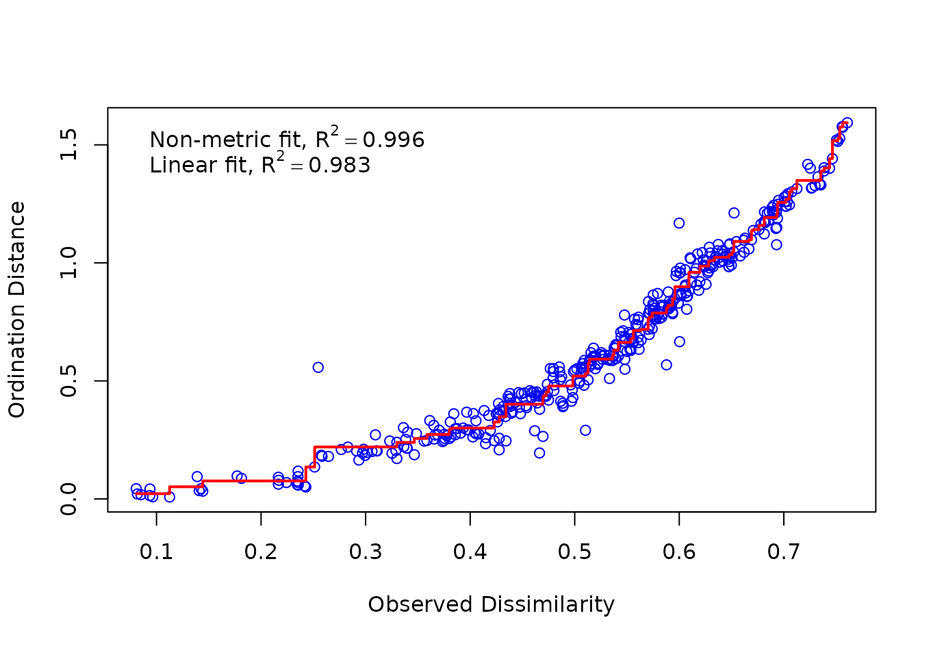

A plot of ordination distances and monotone or linear fit line against original dissimilarities.

Now, we’ll create a function for a) ordinate and b) plot. This way we’ll be able to plot for different subsets of taxa at the same time.

plot_nmds <- function(x, ...){
  y <-ordinate(x, method = "NMDS", distance = "bray")
  plot_ordination(x, y, ...)+
  geom_point(size=3)+
  theme(
    legend.title = element_blank(),
    legend.position = "right"
  )+
  stat_ellipse()
}

nmds <- list(
  all = plot_nmds(
    physeq_rel,type ="samples", color = "layer",shape = "layer"
    ),
  phyla = physeq_rel |>
    tax_glom(taxrank = "Phylum", NArm = FALSE) |>
    plot_nmds(
      type ="samples", color = "layer", shape = "layer"
      ),
  class = physeq_rel |>
    tax_glom(taxrank = "Class", NArm = FALSE) |>
    plot_nmds(
      type ="samples", color = "layer", shape = "layer"
      )
)
#> Wisconsin double standardization
#> Run 0 stress 0.0634 
#> Run 1 stress 0.0634 
#> ... Procrustes: rmse 3.99e-05  max resid 0.000112 
#> ... Similar to previous best
#> Run 2 stress 0.0894 
#> Run 3 stress 0.0841 
#> Run 4 stress 0.0908 
#> Run 5 stress 0.0634 
#> ... New best solution
#> ... Procrustes: rmse 1.15e-05  max resid 3.01e-05 
#> ... Similar to previous best
#> Run 6 stress 0.0634 
#> ... Procrustes: rmse 2.55e-05  max resid 6.96e-05 
#> ... Similar to previous best
#> Run 7 stress 0.0634 
#> ... New best solution
#> ... Procrustes: rmse 5.26e-06  max resid 1.21e-05 
#> ... Similar to previous best
#> Run 8 stress 0.0634 
#> ... Procrustes: rmse 1.95e-05  max resid 4.93e-05 
#> ... Similar to previous best
#> Run 9 stress 0.0848 
#> Run 10 stress 0.1 
#> Run 11 stress 0.0634 
#> ... Procrustes: rmse 1.3e-05  max resid 3.28e-05 
#> ... Similar to previous best
#> Run 12 stress 0.0634 
#> ... Procrustes: rmse 1.23e-05  max resid 3.34e-05 
#> ... Similar to previous best
#> Run 13 stress 0.0634 
#> ... Procrustes: rmse 1.37e-05  max resid 3.63e-05 
#> ... Similar to previous best
#> Run 14 stress 0.0821 
#> Run 15 stress 0.0634 
#> ... Procrustes: rmse 4.4e-05  max resid 0.000118 
#> ... Similar to previous best
#> Run 16 stress 0.0634 
#> ... Procrustes: rmse 6.43e-05  max resid 0.000177 
#> ... Similar to previous best
#> Run 17 stress 0.0898 
#> Run 18 stress 0.0821 
#> Run 19 stress 0.0634 
#> ... New best solution
#> ... Procrustes: rmse 3.45e-06  max resid 9.16e-06 
#> ... Similar to previous best
#> Run 20 stress 0.0634 
#> ... Procrustes: rmse 1.44e-05  max resid 3.6e-05 
#> ... Similar to previous best
#> *** Best solution repeated 2 times
#> Square root transformation
#> Wisconsin double standardization
#> Run 0 stress 0.0653 
#> Run 1 stress 0.0653 
#> ... Procrustes: rmse 7.76e-06  max resid 3.29e-05 
#> ... Similar to previous best
#> Run 2 stress 0.112 
#> Run 3 stress 0.0877 
#> Run 4 stress 0.0653 
#> ... Procrustes: rmse 4.04e-06  max resid 1.4e-05 
#> ... Similar to previous best
#> Run 5 stress 0.0653 
#> ... Procrustes: rmse 8.45e-06  max resid 3.45e-05 
#> ... Similar to previous best
#> Run 6 stress 0.112 
#> Run 7 stress 0.116 
#> Run 8 stress 0.0877 
#> Run 9 stress 0.112 
#> Run 10 stress 0.0653 
#> ... New best solution
#> ... Procrustes: rmse 1.59e-06  max resid 6.39e-06 
#> ... Similar to previous best
#> Run 11 stress 0.0653 
#> ... Procrustes: rmse 3.55e-06  max resid 1.52e-05 
#> ... Similar to previous best
#> Run 12 stress 0.0877 
#> Run 13 stress 0.0653 
#> ... Procrustes: rmse 3.28e-06  max resid 1.13e-05 
#> ... Similar to previous best
#> Run 14 stress 0.0653 
#> ... Procrustes: rmse 3.41e-06  max resid 1.4e-05 
#> ... Similar to previous best
#> Run 15 stress 0.112 
#> Run 16 stress 0.128 
#> Run 17 stress 0.0653 
#> ... Procrustes: rmse 1.42e-05  max resid 5.79e-05 
#> ... Similar to previous best
#> Run 18 stress 0.0653 
#> ... Procrustes: rmse 1.71e-05  max resid 7.43e-05 
#> ... Similar to previous best
#> Run 19 stress 0.0874 
#> Run 20 stress 0.112 
#> *** Best solution repeated 6 times
#> Square root transformation
#> Wisconsin double standardization
#> Run 0 stress 0.0983 
#> Run 1 stress 0.0959 
#> ... New best solution
#> ... Procrustes: rmse 0.0844  max resid 0.361 
#> Run 2 stress 0.103 
#> Run 3 stress 0.0886 
#> ... New best solution
#> ... Procrustes: rmse 0.0856  max resid 0.368 
#> Run 4 stress 0.0717 
#> ... New best solution
#> ... Procrustes: rmse 0.102  max resid 0.357 
#> Run 5 stress 0.087 
#> Run 6 stress 0.0717 
#> ... Procrustes: rmse 0.000102  max resid 0.000433 
#> ... Similar to previous best
#> Run 7 stress 0.0717 
#> ... Procrustes: rmse 0.00526  max resid 0.0225 
#> Run 8 stress 0.087 
#> Run 9 stress 0.0865 
#> Run 10 stress 0.105 
#> Run 11 stress 0.0717 
#> ... New best solution
#> ... Procrustes: rmse 1.86e-05  max resid 7.67e-05 
#> ... Similar to previous best
#> Run 12 stress 0.095 
#> Run 13 stress 0.105 
#> Run 14 stress 0.0865 
#> Run 15 stress 0.1 
#> Run 16 stress 0.0717 
#> ... Procrustes: rmse 0.00525  max resid 0.0225 
#> Run 17 stress 0.087 
#> Run 18 stress 0.087 
#> Run 19 stress 0.085 
#> Run 20 stress 0.0983 
#> *** Best solution repeated 1 times

You can plot each plot individually:

nmds$all

Or use plot_grid for a list of plots:

plot_grid(plotlist = nmds)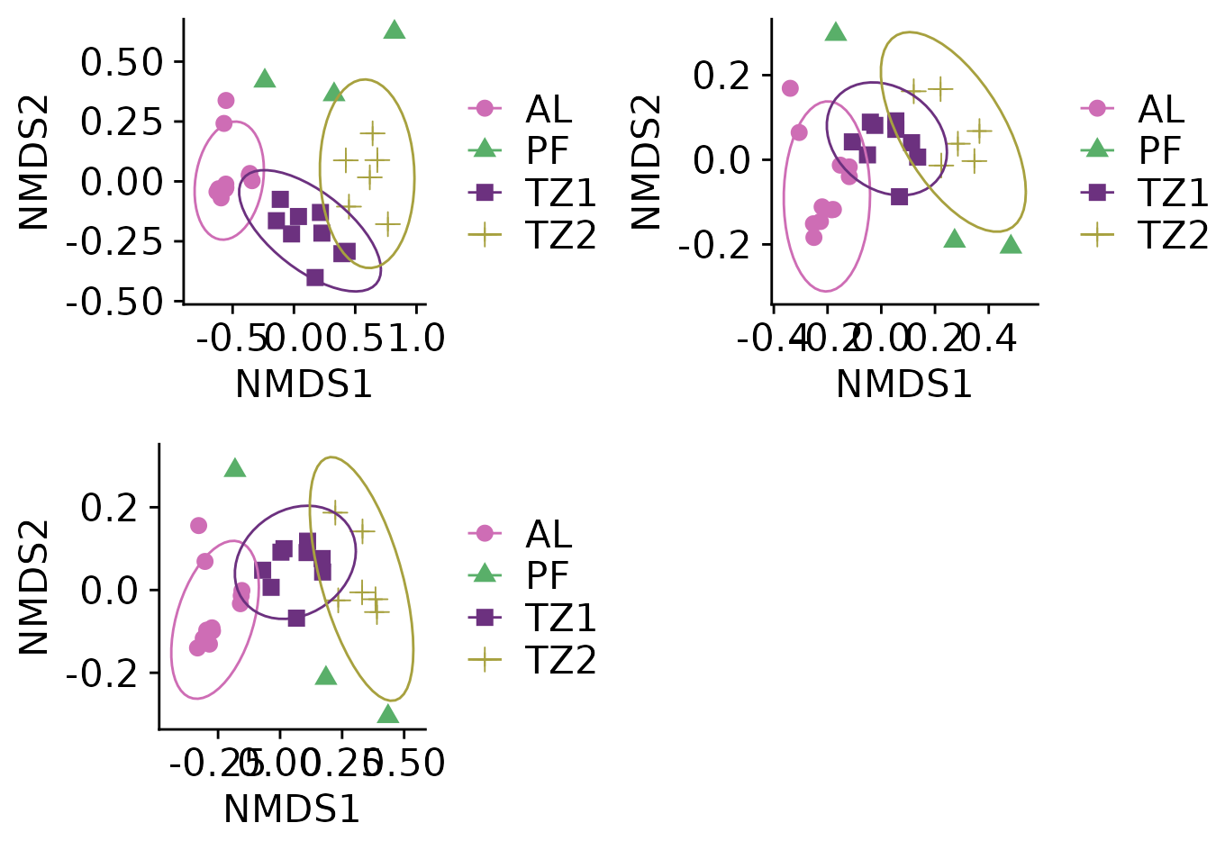

Richness plot

###----Richness all----

richness_plot <- plot_richness(
  physeq, x="layer", color =  "depth",
  measures=c("Observed","Shannon","Simpson","InvSimpson")
  )
richness_plot <- richness_plot + geom_boxplot(
  data = richness_plot$data, aes(color = NULL), alpha = 0.05)+
  theme(
    legend.title = element_blank(),
    legend.position = "right"
  )
richness_plot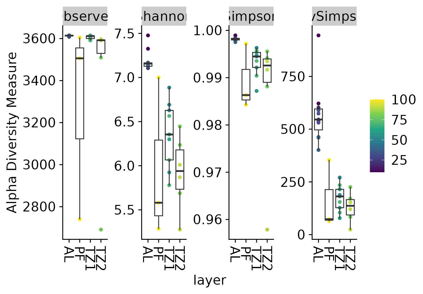

Stacked bar plots

physeq_mean_rel_phylum <- physeq_mean_rel |>
  tax_glom(taxrank = "Phylum") |>
  transform_sample_counts(function(x) x/sum(x)*100)

Since we get too many phyla to plot in a stacked barplot, we will filter the low abundant ones and put them into one category. To do this, we will use the tidyverse again. First, we will create a normal data frame out of the phyloseq object and then add another column where all taxa with abundance lower than 3% will be renamed to “< 3%”.

physeq_mean_rel_phylumDF <- physeq_mean_rel_phylum |>
  #transform phyloseq object to a data frame (DF)
  psmelt()|>
  #make the phyla characters, not factors
  mutate(Phylum = as.character(Phylum))|>
  #there are some reads that were assigned only to the kingdom level, 
  # i.e. NA on the phylum level, so we will rename them
  mutate(
    Phylum = replace(Phylum, Phylum == "NA", "unassigned"),
    Phylum2 = replace(Phylum, Abundance < 3, "< 3%")
    )|>
  #reorder the phyla so that they are stacked according to abundance
  mutate(
    Phylum2 = reorder(Phylum2, Abundance)
  )

Now, we plot the stacked plot. You can change colors editing function get_wants_hue. Default is optimized for colorblindness.

n_phyla <- length(levels(physeq_mean_rel_phylumDF$Phylum2))

stacked_plot <- physeq_mean_rel_phylumDF |>
  ggplot(aes(depth, Abundance, fill=Phylum2)) +
  geom_bar(stat = "identity") +
  labs(x= "depth [cm]",y= "Relative abundance [%]",
     fill= "Phyla")+
  scale_fill_manual(values = get_wants_hue(n_phyla))+
  theme(legend.position="bottom") +
  scale_x_continuous(breaks = seq(10, 100, 10))
stacked_plot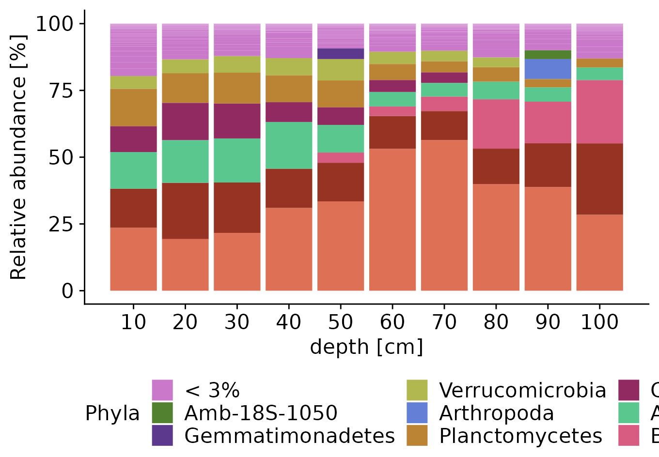

You can obtain figures with more than one plot using plot_grid. For example:

https://wilkelab.org/cowplot/articles/plot_grid.html

final <- plot_grid(
  stacked_plot, richness_plot,nrow = 2,labels = c("A", "B")
  )
final

ANOVA

First, create objects for microbiome package:

otu_microbiome <- microbiome::abundances(physeq)
meta_microbiome <- microbiome::meta(physeq)


otu_microbiome |> head() |> knitr::kable()

	TK20-2	TK20-3	TK20-4	TK20-5	TK20-6	TK20-7	TK20-8	TK20-9	TK20-10	TK20-11	TK20-12	TK20-13	TK20-14	TK20-15	TK20-16	TK20-17	TK20-18	TK20-19	TK20-20	TK20-21	TK20-22	TK20-23	TK20-24	TK20-25	TK20-26	TK20-27	TK20-28	TK20-29	TK20-30
0319-6G20	344	338	872	944	187	83	17	47	6	412	774	355	4769	992	2959	18	1	30	0	139	646	363	962	956	884	246	0	23	70
Kineosporia	5776	14725	4922	3000	3304	646	298	448	401	10733	5590	9648	80899	8926	783	234	65	190	71	13144	6740	9200	4332	4624	911	186	4	149	412
OM1clade	4	5	3	2	9	295	4380	10308	7	16	13	4	29	0	23	167	1190	5087	3	3	15	11	10	9	1	5	5	8557	16
Ca.Parcubacteria	83	73	56	11	18	64	125	306	1	84	181	61	387	4	83	42	23	156	0	36	117	52	113	25	16	63	2	43	9
Nitrosomonadaceae	1798	886	2251	3176	437	1598	2589	7291	4790	261	3532	785	14943	1829	8676	1151	2294	3138	8	174	2186	555	2508	2096	3313	2074	65	2503	2538
Ca.Solibacter	292	595	540	29	89	75	12	63	11	234	388	362	2452	18	254	28	143	31	0	231	318	414	708	74	25	38	14	67	27

meta_microbiome |> knitr::kable()

	layer	age	pH	depth
TK20-2	AL	AY	4.02	20
TK20-3	AL	AY	4.29	30
TK20-4	AL	AY	4.25	40
TK20-5	TZ1	AM	4.64	50
TK20-6	TZ1	AM	4.13	60
TK20-7	TZ1	AO	4.86	70
TK20-8	TZ2	AO	4.48	80
TK20-9	TZ2	AO	4.57	90
TK20-10	PF	AO	4.91	100
TK20-11	AL	AY	4.22	10
TK20-12	AL	AY	4.02	20
TK20-13	AL	AY	4.29	30
TK20-14	AL	AY	4.25	40
TK20-15	TZ1	AM	4.64	50
TK20-16	TZ1	AM	4.13	60
TK20-17	TZ1	AO	4.86	70
TK20-18	TZ2	AO	4.48	80
TK20-19	TZ2	AO	4.57	90
TK20-20	PF	AO	4.91	100
TK20-21	AL	AY	4.22	10
TK20-22	AL	AY	4.02	20
TK20-23	AL	AY	4.29	30
TK20-24	AL	AY	4.25	40
TK20-25	TZ1	AM	4.64	50
TK20-26	TZ1	AM	4.13	60
TK20-27	TZ1	AO	4.86	70
TK20-28	TZ2	AO	4.48	80
TK20-29	TZ2	AO	4.57	90
TK20-30	PF	AO	4.91	100

Now, we use adonis for those variables we are interested. We should probably use adonis2, because adonis have been deprecated.


permanova_depth <- adonis2(
  t(otu_microbiome)~depth,
  data = meta_microbiome,
  permutations=999, method = "bray"
  )
permanova_depth
#> Permutation test for adonis under reduced model
#> Terms added sequentially (first to last)
#> Permutation: free
#> Number of permutations: 999
#> 
#> adonis2(formula = t(otu_microbiome) ~ depth, data = meta_microbiome, permutations = 999, method = "bray")
#>          Df SumOfSqs    R2    F Pr(>F)    
#> depth     1     1.91 0.255 9.26  0.001 ***
#> Residual 27     5.56 0.745                
#> Total    28     7.46 1.000                
#> ---
#> Signif. codes:  0 '***' 0.001 '**' 0.01 '*' 0.05 '.' 0.1 ' ' 1

Now layer:

permanova_layer <- adonis2(
  t(otu_microbiome)~layer,
  data = meta_microbiome,
  permutations=999, method = "bray"
  )
permanova_layer
#> Permutation test for adonis under reduced model
#> Terms added sequentially (first to last)
#> Permutation: free
#> Number of permutations: 999
#> 
#> adonis2(formula = t(otu_microbiome) ~ layer, data = meta_microbiome, permutations = 999, method = "bray")
#>          Df SumOfSqs    R2    F Pr(>F)    
#> layer     3     3.17 0.425 6.15  0.001 ***
#> Residual 25     4.30 0.575                
#> Total    28     7.46 1.000                
#> ---
#> Signif. codes:  0 '***' 0.001 '**' 0.01 '*' 0.05 '.' 0.1 ' ' 1

If you have several “models”, consider a more general approach using lists:

adonis2_formulas <- list(
  layer = t(otu_microbiome)~layer,
  depth = t(otu_microbiome)~depth
)
permanovas <- adonis2_formulas |>
  map(
    adonis2, data = meta_microbiome,
    permutations=999, method = "bray"
    )
permanovas$layer
#> Permutation test for adonis under reduced model
#> Terms added sequentially (first to last)
#> Permutation: free
#> Number of permutations: 999
#> 
#> .f(formula = .x[[i]], data = ..1, permutations = 999, method = "bray")
#>          Df SumOfSqs    R2    F Pr(>F)    
#> layer     3     3.17 0.425 6.15  0.001 ***
#> Residual 25     4.30 0.575                
#> Total    28     7.46 1.000                
#> ---
#> Signif. codes:  0 '***' 0.001 '**' 0.01 '*' 0.05 '.' 0.1 ' ' 1
permanovas$depth
#> Permutation test for adonis under reduced model
#> Terms added sequentially (first to last)
#> Permutation: free
#> Number of permutations: 999
#> 
#> .f(formula = .x[[i]], data = ..1, permutations = 999, method = "bray")
#>          Df SumOfSqs    R2    F Pr(>F)    
#> depth     1     1.91 0.255 9.26  0.001 ***
#> Residual 27     5.56 0.745                
#> Total    28     7.46 1.000                
#> ---
#> Signif. codes:  0 '***' 0.001 '**' 0.01 '*' 0.05 '.' 0.1 ' ' 1

Multivariate homogeneity of groups dispersions

# Calculate distance
dist <- vegan::vegdist(t(otu_microbiome), method="bray")
# betadisper is a multivariate analogue of Levene's test for homogeneity of variances
mod_layer <- vegan::betadisper(
  dist, meta_microbiome$layer, type="centroid"
  )
mod_layer$layer <- meta_microbiome$layer

TukeyHSD

(tukey_test <- TukeyHSD(mod_layer))
#>   Tukey multiple comparisons of means
#>     95% family-wise confidence level
#> 
#> Fit: aov(formula = distances ~ group, data = df)
#> 
#> $group
#>             diff    lwr   upr p adj
#> PF-AL    0.12407 -0.111 0.359 0.480
#> TZ1-AL   0.05798 -0.104 0.220 0.760
#> TZ2-AL   0.05981 -0.123 0.243 0.806
#> TZ1-PF  -0.06609 -0.307 0.174 0.873
#> TZ2-PF  -0.06426 -0.319 0.191 0.899
#> TZ2-TZ1  0.00183 -0.188 0.192 1.000

plot(tukey_test)

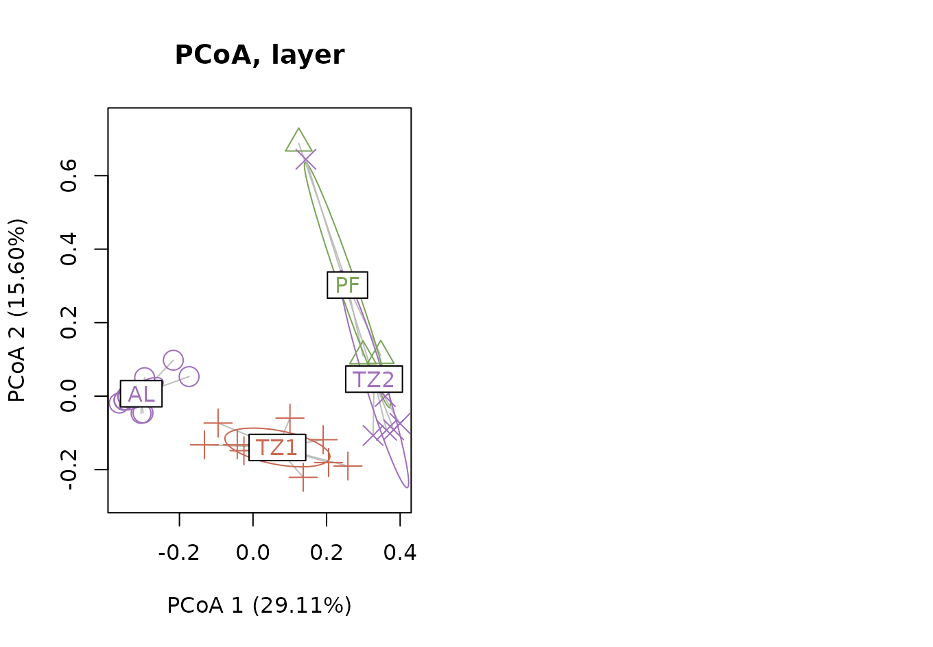
PCoA with variance in axis

get_variance <- function(mod, number, digits = 2){
  variance <- mod$eig[number]/sum(mod$eig)*100
  variance |>
    round(digits) |> 
    format(nsmall = digits)
}
x_label <- paste0('PCoA 1 (', get_variance(mod_layer, 1),'%)')
y_label <- paste0('PCoA 2 (', get_variance(mod_layer, 2),'%)')

par(mfrow = c(1,2))
plot(
  mod_layer,  hull=FALSE, ellipse=TRUE,
  main = "PCoA, layer", sub=NULL,
  col= RauENVS::get_wants_hue(seed = 10, n = 3, palette = "default"),
  cex=2, lwd=1,
  xlab = x_label,
  ylab = y_label
  ) #+

Boxplot of distances with pvalues from Tukey Test

We can add p-values from to the box plot of the distances:


get_pos_whisker <- function(x){
  # Calculate whisker position
  hinge <- as.numeric(quantile(x, probs = 0.75))
  upper_max <- hinge +IQR(x)*1.5 
  x |> 
    keep(~ . < upper_max) |>
    max()
}
# Calculate label position
pos <-  c(
  by(mod_layer$distances, mod_layer$group, get_pos_whisker)
  )

# You can run the next line for calculating automatically the
# labels based in p-values.
tukey_label <-   data.frame(
    label = rownames(tukey_test$group)[which(
      tukey_test$group[,'p adj']< 0.05
      )]
  ) |>
  separate(label,sep = '-', into = c('from', 'to'),remove = T) %$%
  data.frame(from = c(from, to), to = c(to, from)) |>
  group_by(from)|>
  summarise(label = paste0(to, collapse = ','))|>
  column_to_rownames('from')|>
  pull(label)

# However, for this data, there is no significance difference 
# between groups. We can still plot those labels as example:

custom_label <- c('A', 'V', 'AV', 'T2')

tibble(
  distances = mod_layer$distances,
  group = mod_layer$group,
) |>
  ggplot(aes(x = group, y = distances, fill = group))+
  geom_boxplot()+
  geom_text(
    data = data.frame(
      distances = pos,group = names(pos),label = custom_label
      ),
    aes(label = label),
    hjust = -1, vjust = -0.5
    )+
  xlab('Layer')+ylab('Distance to Centroid')+
  theme(legend.position = 'None')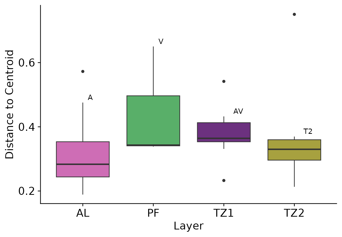

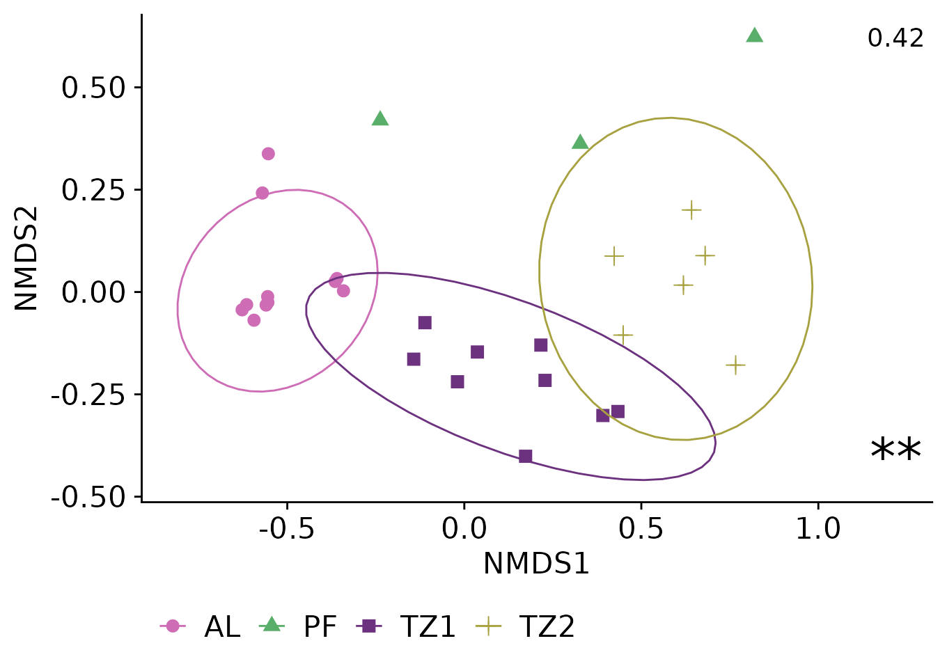
Annotating NMDS with information from permanova

“Numbers on the top indicate the stress values.
Asterisks represent the significance level of PERMANOVA (∗adjusted P < 0.05 or ∗∗adjusted P < 0.01)”

First, we extract information from permanova

(
  r2_label <- permanova_layer$R2[[1]] |>
  round(2) |>
  format(nsmall = 2)
)
#> [1] "0.42"
(
p_value_label <- permanova_layer$`Pr(>F)`[[1]]%>%
  {case_when(
    . < 0.01 ~ "**",
    . < 0.05 ~ "*",
    . >= 0.05 ~ "",
    )}
)
#> [1] "**"

original_plot <- plot_ordination(
  physeq_rel, physeq_nmds,
  type ="samples", color = "layer",shape = "layer"
  )+
  geom_point(size=3)+
  stat_ellipse()+
  theme(
    legend.position="bottom",
    legend.title = element_blank()
    )

original_plot +
  annotate(
    geom="text",
    x = max(original_plot$data$NMDS1) + 0.4,
    y = max(original_plot$data$NMDS2),
    label= r2_label,
    size = 5
    )+
  annotate(
    geom="text",
    x = max(original_plot$data$NMDS1) + 0.4,
    y = min(original_plot$data$NMDS2),
    label= p_value_label,
    size = 10
    )

AU-ENVS Bioinformatics

Read your data

Read metadata table

Read OTU table

Read OTU table

Sanity check

Preprocess your data

Transform into phyloseq object

Dealing with taxonomic categories

Data cleaning

Making unique OTU labels

Transform sample counts

Inspect data

Data analysis

Perform an ordination using Nonmetric Multidimensional Scaling

Goodness of Fit and Shepard Plot for Nonmetric Multidimensional Scaling

Richness plot

Stacked bar plots

ANOVA

Multivariate homogeneity of groups dispersions

TukeyHSD

PCoA with variance in axis

Boxplot of distances with pvalues from Tukey Test

Annotating NMDS with information from permanova